Quick start example of basic MCycle features ¶

Contents

Quick start example of basic MCycle features

This quickstart example goes through creating a basic organic Rankine cycle and demonstrates some basic MCycle functions, including:

setting MCycle defaults,

creating flowstates, components and cycles,

plotting a cycle,

printing a cycle summary

using the size and run methods to analyse a component

This script should be copied and run from your local directory. Keyword arguments have been specified throughout this example for clarity however in practice these are not strictly required.

Setting up MCycle ¶

Having correctly installed MCycle from either the source code or pip (see installation notes), MCycle and CoolProp must first be imported.:

>>> import mcycle as mc
>>> import CoolProp as CP

Next, we change a couple of the MCycle defaults to our liking. The check() function should be executed after changing defaults to ensure the new value is valid and to run any required backend functions to register the change.

>>> mc.defaults.PLOT_DIR = "" # will not create a new folder for plots
>>> mc.defaults.PLOT_DPI = 200
>>> mc.defaults.check()

Creating flowstates ¶

To represent the working fluid of the cycle, we must create a FlowState object. The mass flow rate and initial state conditions do not need to be defined, as they will be set later by the cycle parameters, but for the sake of demonstrating the full constructor, we can assign some arbitrary values. Note that iphase = PHASE_NOT_IMPOSED is used when the flow phase does not explicitly need to be defined. FlowState objects will use the CoolProp backend specified by the defaults.COOLPROP_EOS attribute, which defaults to "HEOS".

>>> wf = mc.FlowState(fluid="R245fa", m=1.0, inputPair=mc.PT_INPUTS, input1=mc.atm2Pa(1), input2=298, iphase=mc.PHASE_NOT_IMPOSED)

Printing flowstate summaries ¶

The summary() method is quick way to print a customisable summary of a flowstate.

>>> wf.summary(title='Working fluid')
Working fluid summary
=====================
T() = 2.9800e+02 [K]
p() = 1.0132e+05 [Pa]
rho() = 5.6918e+00 [Kg/m^3]
h() = 4.2539e+05 [J/Kg]
s() = 1.7835e+03 [J/Kg.K]
cp() = 8.8817e+02 [J/Kg.K]
visc() = 1.1810e-05 [N.s/m^2]
k() = 1.5704e-02 [W/m.K]
Pr() = 6.6798e-01
x() = -1.0000e+00

Creating components ¶

Before creating the cycle, we must create the individual Component objects. An organic Rankine cycle requires an expander, condenser, compressor and evaporator. For this example we will use the most basic models for each component. Again, many of the attributes will be set later by the cycle parameters, including the incoming and outgoing flowstates, but we will assign some of them arbitrary values here for demonstration purposes.

>>> exp = mc.ExpBasic(pRatio=1, efficiencyIsentropic=0.9, sizeAttr="pRatio")
>>> cond = mc.ClrBasic(constraint=mc.CONSTANT_P, QCool=1, efficiencyThermal=1.0, sizeAttr="Q")
>>> comp = mc.CompBasic(pRatio=1, efficiencyIsentropic=0.85, sizeAttr="pRatio")
>>> evap = mc.HtrBasic(constraint=mc.CONSTANT_P, QHeat=1, efficiencyThermal=1.0, sizeAttr="Q")

Printing component summaries ¶

The summary() method is quick way to print a customisable summary of a component. As the components do not have flowstates yet, we will not include information for any flowstates in the summary.

>>> exp.summary(propertyKeys='all', flowKeys='all', title="Expander")
Expander summary
================
Notes: No notes/model info.
pRatio = 1.0000e+00
effIsentropic = 9.0000e-01
ambient = None
mWf not yet defined pIn not yet defined pOut not yet defined POut() = 0.0000e+00 [W]

flowstate not defined

flowstate not defined

Creating cycles ¶

The RankineBasic object can now be created. We will also define the design cycle parameters which are required by the size() method. As the condensing temperature TCond() is a property computed from the condesing pressure, we define it after constructing the cycle using the update() method. We will use the default Config by not specifying config in the constructor (we could also set it to the value None).

>>> cycle = mc.RankineBasic(wf=wf, evap=evap, exp=exp, cond=cond, comp=comp, config=None)
>>> cycle.update({"pEvap": mc.bar2Pa(10), "superheat": 10., "TCond": mc.degC2K(25), "subcool": 5.})

Plotting cycles ¶

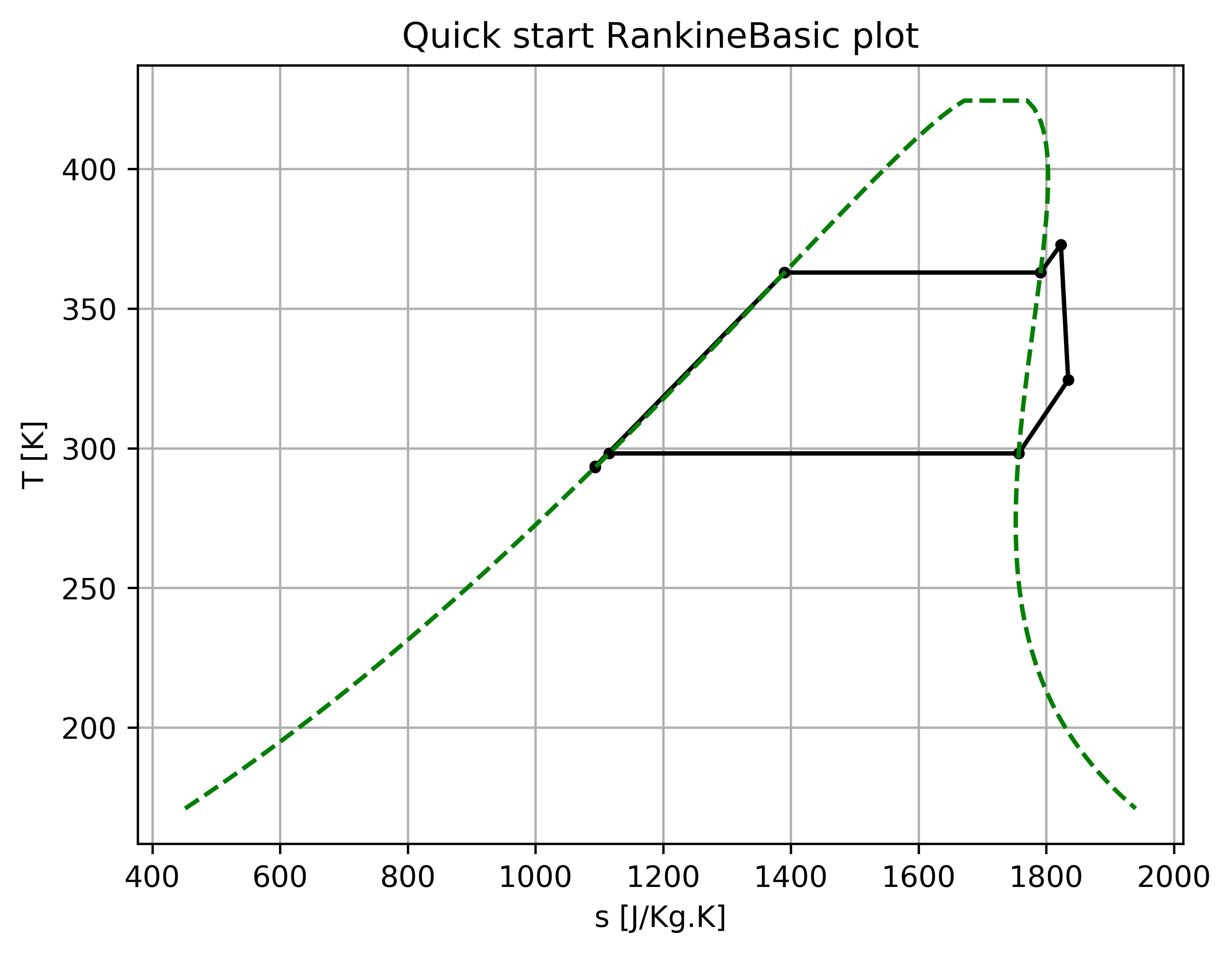
With the cycle and its components now set up, we can start by plotting the cycle at the design conditions on a temperature-entropy diagram using the plot() method. Currently, the cycle has been constructed, but the flowstates of the cycle components still have not been initialised. Although the size() method takes care of this, with more complex cycle components, this method may be time-consuming. As a shortcut, the sizeSetup() method was created, which initialises all cycle flowstates to design conditions, but does not proceed to size each of the components. We will also specify not to unitise the evaporator or condenser, although for this example this would not occur anyway as we have not used components that require unitisation.

>>> cycle.sizeSetup(unitiseEvap=False, unitiseCond=False)
>>> cycle.plot(graph='Ts', # either 'Ts' or 'ph'
               title='Quick start RankineBasic plot', # graph title
               satCurve=True, # display saturation curve
               newFig=True, # create a new figure
               show=False, # show the figure
               savefig=True, # save the figure
               savefig_name='quickstart_plot_RankineBasic',
               plot_folder='')

This produces the following graph.

Printing cycle summaries ¶

Although plotting the cycle is a great visual representation of the cycle, often a more in depth summary is required. Here we will size the cycle to the design parameters and print a complete summary of the cycle. The size() method, as mentioned above, calls the size() method of each component of the cycle. The sizeAttr attribute determines which component attribute will be sized, while the sizeBounds attribute defines the bounds containing the solution (not all components require this for their size() method). For now, we will use the default values for each of the cycle components.

>>> cycle.size()

Now, to print the cycle summary, we simply use the summary() method, selecting to print all cycle component and flowstate summaries.

>>> cycle.summary(printSummary=True, propertyKeys='all', cycleStateKeys='all', componentKeys='all', title="Quick start RankineBasic cycle")

This prints the following output in rST format:

Quick start RankineBasic cycle summary
======================================
working fluid: R245fa
pEvap = 1.0000e+06 [Pa]
superheat = 1.0000e+01 [K]
pCond = 1.4858e+05 [Pa]
subcool = 5.0000e+00 [K]

Properties
----------
mWf = 1.0000e+00 [Kg/s]
QIn() = 2.5446e+05 [W]
QOut() = 2.2194e+05 [W]
PIn() = 7.4039e+02 [W]
POut() = 3.3256e+04 [W]
effThermal() = 1.2778e-01
effExergy() = nan
IComp() = nan [W]
IEvap() = nan [W]
IExp() = nan [W]
ICond() = nan [W]

evap summary
------------
Notes: No notes/model info.
Q = 2.5446e+05 [W]
effThermal = 1.0000e+00
ambient = None

exp summary
-----------
Notes: No notes/model info.
pRatio = 6.7303e+00
effIsentropic = 9.0000e-01
ambient = None

cond summary
------------
Notes: No notes/model info.
Q = 2.2194e+05 [W]
effThermal = 1.0000e+00
ambient = None

comp summary
------------
Notes: No notes/model info.
pRatio = 6.7303e+00
effIsentropic = 8.5000e-01
ambient = None

state1 summary
--------------
T() = 2.9351e+02 [K]
p() = 1.0000e+06 [Pa]
rho() = 1.3535e+03 [Kg/m^3]
h() = 2.2717e+05 [J/Kg]
s() = 1.0937e+03 [J/Kg.K]
cp() = 1.3031e+03 [J/Kg.K]
visc() = 4.2221e-04 [N.s/m^2]
k() = 9.3756e-02 [W/m.K]
Pr() = 5.8684e+00
x() = -1.0000e+00

state20 summary
---------------
T() = 3.6290e+02 [K]
p() = 1.0000e+06 [Pa]
rho() = 1.1347e+03 [Kg/m^3]
h() = 3.2443e+05 [J/Kg]
s() = 1.3903e+03 [J/Kg.K]
cp() = 1.5345e+03 [J/Kg.K]
visc() = 1.8747e-04 [N.s/m^2]
k() = 7.3074e-02 [W/m.K]
Pr() = 3.9368e+00
x() = 0.0000e+00

state21 summary
---------------
T() = 3.6290e+02 [K]
p() = 1.0000e+06 [Pa]
rho() = 5.6000e+01 [Kg/m^3]
h() = 4.6986e+05 [J/Kg]
s() = 1.7911e+03 [J/Kg.K]
cp() = 1.1907e+03 [J/Kg.K]
visc() = 1.4900e-05 [N.s/m^2]
k() = 2.2481e-02 [W/m.K]
Pr() = 7.8917e-01
x() = 1.0000e+00

state3 summary
--------------
T() = 3.7290e+02 [K]
p() = 1.0000e+06 [Pa]
rho() = 5.2741e+01 [Kg/m^3]
h() = 4.8162e+05 [J/Kg]
s() = 1.8231e+03 [J/Kg.K]
cp() = 1.1649e+03 [J/Kg.K]
visc() = 1.5219e-05 [N.s/m^2]
k() = 2.3235e-02 [W/m.K]
Pr() = 7.6306e-01
x() = -1.0000e+00

state4 summary
--------------
T() = 3.2440e+02 [K]
p() = 1.4858e+05 [Pa]
rho() = 7.6848e+00 [Kg/m^3]
h() = 4.4837e+05 [J/Kg]
s() = 1.8345e+03 [J/Kg.K]
cp() = 9.3769e+02 [J/Kg.K]
visc() = 1.2887e-05 [N.s/m^2]
k() = 1.8020e-02 [W/m.K]
Pr() = 6.7062e-01
x() = -1.0000e+00

state51 summary
---------------
T() = 2.9815e+02 [K]
p() = 1.4858e+05 [Pa]
rho() = 8.5033e+00 [Kg/m^3]
h() = 4.2421e+05 [J/Kg]
s() = 1.7569e+03 [J/Kg.K]
cp() = 9.0375e+02 [J/Kg.K]
visc() = 1.1826e-05 [N.s/m^2]
k() = 1.5749e-02 [W/m.K]
Pr() = 6.7860e-01
x() = 1.0000e+00

state50 summary
---------------
T() = 2.9815e+02 [K]
p() = 1.4858e+05 [Pa]
rho() = 1.3385e+03 [Kg/m^3]
h() = 2.3298e+05 [J/Kg]
s() = 1.1155e+03 [J/Kg.K]
cp() = 1.3168e+03 [J/Kg.K]
visc() = 3.9480e-04 [N.s/m^2]
k() = 9.1962e-02 [W/m.K]
Pr() = 5.6531e+00
x() = 0.0000e+00

state6 summary
--------------
T() = 2.9315e+02 [K]
p() = 1.4858e+05 [Pa]
rho() = 1.3520e+03 [Kg/m^3]
h() = 2.2643e+05 [J/Kg]
s() = 1.0933e+03 [J/Kg.K]
cp() = 1.3049e+03 [J/Kg.K]
visc() = 4.1907e-04 [N.s/m^2]
k() = 9.3477e-02 [W/m.K]
Pr() = 5.8501e+00
x() = -1.0000e+00

An mcycle.log file will also be created in the working directory, as certain cycle properties (exergy destruction values: IEvap(), IExp(), ICond(), IComp()) are not valid with the basic component classes.

Running a cycle at off-design conditions ¶

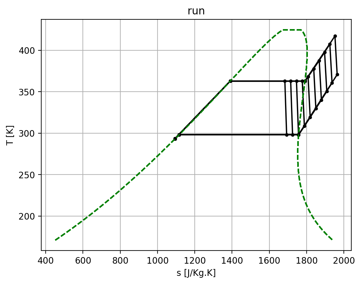
Finally, we’ll use the run() method to analyse the evaporator at off-design conditions. We will vary the heat added to the cycle via the evaporator and analyse how this affects the maximum temperature (at state3) and thermal efficiency effThermal(). We start by setting up the cycle to design conditions using sizeSetup() and defining the bounds of the heat addition we will consider, in this case 0.8x to 1.2x the design value. Next we create empty lists for storing the results and as we would like to also plot the results, we also create a flag to append all plots on one figure instead of creating a new figure each time.

>>> cycle.sizeSetup(False, False)
>>> Qfraction_vals = np.linspace(0.8, 1.2, 11, True)
>>> Q_vals = Qfraction_vals * cycle.QIn()

>>> state3_vals = []
>>> effThermal_vals = []

>>> newFigFlag = True # append to one figure

Now we can go ahead and run the evaporator. While we could use the cycle run() method which runs each of the components, instead we will just run the evaporator and expander. As running the evaporator affects the state3 flowstate which is shared byt he evaporator and expander, we must remember to set it using set_state3() which ensures all affected components now have the updated object. Similarly, we must now re-run the expander as its incoming working fluid flowstate has now changed and also use set_state4() to ensure the changes are passed on to the condenser. We save state3 and efficiencyThermal() into the storage lists and plot up the results. We will also plot the results into a table for easier viewing of the values.:

>>> for Q in Q_vals:
        cycle.evap.Q = Q

        cycle.evap.run()
        cycle.set_state3(cycle.evap.flowOutWf)

        cycle.exp.run()
        cycle.set_state4(cycle.exp.flowOutWf)

        state3_vals.append(cycle.state3)
        effThermal_vals.append(cycle.efficiencyThermal())
        cycle.plot(
            graph='Ts',  # either 'Ts' or 'ph'
            title='run',  # graph title
            satCurve=True,  # display saturation curve
            newFig=newFigFlag,  # append to existing figure
            show=False,  # show the figure
            savefig=True,  # save the figure
            savefig_name='quickstart_run')
        newFigFlag = False

>>> print("Q/Q_design | state3.T() | state3.x() | efficiencyThermal")
>>> for i in range(len(Qfraction_vals)):
        print("{:1.2f} | {:3.2f} | {: 2.2f} | {:1.4f}".format(Qfraction_vals[i], state3_vals[i].T(), state3_vals[i].x(), effThermal_vals[i]))

This produces the following graph and output.

Running RankineBasic at off-design conditions

Q/Q_design | state3.T() | state3.x() | efficiencyThermal()
80 | 362.90 |  0.73 | 0.1223
84 | 362.90 |  0.80 | 0.1241
88 | 362.90 |  0.87 | 0.1257
92 | 362.90 |  0.94 | 0.1272
96 | 364.23 | -1.00 | 0.1277
00 | 372.90 | -1.00 | 0.1278
04 | 381.69 | -1.00 | 0.1277
08 | 390.55 | -1.00 | 0.1274
12 | 399.44 | -1.00 | 0.1270
16 | 408.33 | -1.00 | 0.1266
20 | 417.21 | -1.00 | 0.1260

Conclusions ¶

This concludes a quick example into some of the main features of mcycle. Check out the other examples or explore the documentation for more advanced features.

Source code¶"""Quick start example of basic MCycle features."""

import mcycle as mc
from math import nan
import CoolProp as CP
import numpy as np

print("Begin quickstart example...")

# ************************************************
# Set MCycle defaults
# ************************************************
print("Set MCycle defaults...")
mc.defaults.PLOT_DIR = ""
mc.defaults.PLOT_DPI = 200
mc.defaults.check()
print("defaults done.")

print("Begin Rankine cycle setup...")
wf = mc.FlowState(
    fluid="R245fa",
    m=1.0,
    inputPair=mc.PT_INPUTS,
    input1=mc.atm2Pa(1),
    input2=298)
print("  - created working fluid")
exp = mc.ExpBasic(pRatio=1, efficiencyIsentropic=0.9, sizeAttr="pRatio")
print("  - created expander")
cond = mc.ClrBasic(constraint=mc.CONSTANT_P, QCool=1, efficiencyThermal=1.0, sizeAttr="Q")
print("  - created condenser")
comp = mc.CompBasic(pRatio=1, efficiencyIsentropic=0.85, sizeAttr="pRatio")
print("  - created compressor")
evap = mc.HtrBasic(constraint=mc.CONSTANT_P, QHeat=1, efficiencyThermal=1.0, sizeAttr="Q")
print("  - created evaporator")
config = mc.Config()
print("  - created configuration object")
cycle = mc.RankineBasic(
    wf=wf, evap=evap, exp=exp, cond=cond, comp=comp, config=config)
cycle.update({
    "pEvap": mc.bar2Pa(10),
    "superheat": 10.,
    "TCond": mc.degC2K(25),
    "subcool": 5.
})
print("  - created cycle")
print("setup done.")


@mc.timer
def plot_cycle():
    cycle.sizeSetup(unitiseEvap=False, unitiseCond=False)
    cycle.plot(
        graph='Ts',  # either 'Ts' or 'ph'
        title='Quick start RankineBasic plot',  # graph title
        satCurve=True,  # display saturation curve
        newFig=True,  # create a new figure
        show=False,  # show the figure
        savefig=True,  # save the figure
        savefig_name='quickstart_plot_RankineBasic')


@mc.timer
def cycle_summary():
    cycle.size()
    cycle.summary(
        printSummary=True,
        propertyKeys='all',
        cycleStateKeys='all',
        componentKeys='all',
        title="Quick start RankineBasic cycle")


@mc.timer
def run_off_design():
    cycle.sizeSetup(False, False)
    Qfraction_vals = np.linspace(0.8, 1.2, 11, True)
    Q_vals = Qfraction_vals * cycle.QIn()

    runLowerBound = cycle.evap.flowInWf.copyUpdateState(
        CP.PQ_INPUTS, cycle.evap.flowInWf.p(), 0.4).h()

    runUpperBound = cycle.evap.flowInWf.copyUpdateState(
        CP.PT_INPUTS, cycle.evap.flowInWf.p(), 420.).h()
    cycle.evap.update({'runBounds': [runLowerBound, runUpperBound]})

    state3_vals = []
    efficiencyThermal_vals = []
    newFigFlag = True
    for QHeat in Q_vals:
        cycle.evap.QHeat = QHeat
        cycle.evap.run()
        cycle.set_state3(cycle.evap.flowOutWf)
        cycle.exp.run()
        cycle.set_state4(cycle.exp.flowOutWf)
        state3_vals.append(cycle.state3)
        efficiencyThermal_vals.append(cycle.efficiencyThermal())
        cycle.plot(
            graph='Ts',  # either 'Ts' or 'ph'
            title='run',  # graph title
            satCurve=True,  # display saturation curve
            newFig=newFigFlag,  # append to existing figure
            show=False,  # show the figure
            savefig=True,  # save the figure
            savefig_name='quickstart_run')
        newFigFlag = False

    print("Q/Q_design | state3.T() | state3.x() | efficiencyThermal()")
    for i in range(len(Qfraction_vals)):
        print("{:1.2f} | {:3.2f} | {: 2.2f} | {:1.4f}".format(
            Qfraction_vals[i], state3_vals[i].T(), state3_vals[i].x(),
            efficiencyThermal_vals[i]))


if __name__ == "__main__":
    plot_cycle()
    cycle_summary()
    run_off_design()

Quick start example of basic MCycle features ¶

Setting up MCycle ¶

Creating flowstates ¶

Printing flowstate summaries ¶

Creating components ¶

Printing component summaries ¶

Creating cycles ¶

Plotting cycles ¶

Printing cycle summaries ¶

Running a cycle at off-design conditions ¶

Conclusions ¶

Source code ¶

Table of Contents

Previous topic

Next topic

This Page